Fit the Quadratic Response Plateau (QRP) model by grid search

Fits the quadratic-plateau (smooth broken-line) model $$f(x) = a + b x + c x^2 \ \text{ if } x \le X_0, \qquad f(x) = a - b^2/(4c) \ \text{ if } x > X_0,$$ with $X_0 = -b/(2c)$. The breakpoint is profiled over a grid: for each candidate $X_0$ the model is linear in the plateau level and the curvature, so it is fit by least squares with no starting values, and the $X_0$ minimizing the residual sum of squares is returned. This mirrors fit_lrp() and avoids the convergence problems of a direct nls fit.

Usage

fit_qrp(
  .data = NULL,
  x = NULL,
  cv = NULL,
  trial = NULL,
  step = 0.001,
  search_range = NULL,
  start = NULL,
  local_min_tol = 0.1,
  bootstrap = FALSE,
  n_boot = 1000,
  conf_level = 0.95,
  weights = FALSE
)

Arguments

.data: optional data frame; when supplied, x/cv/trial are column names.
x, cv: numeric vectors, or column names when .data is a data frame.
trial: optional column name identifying the trial.
step: grid step for the breakpoint search (default 0.001).
search_range: optional c(lower, upper) restricting the breakpoint search; must fall within the data range.
start: optional single breakpoint value. The fit is unchanged, but the result also carries $compat: the local minimum of the basin containing start, i.e. what a gradient-based fitter seeded there would return. Rarely needed for the QRP, whose SSE profile is usually a single smooth basin.
local_min_tol: relative SSE tolerance (default 0.10) deciding which local minima count as competing. Only labelling is affected (the competing column of $local_minima and the stars in print()); the fit never changes, and no warning is issued.
bootstrap: logical; if TRUE, also estimate the uncertainty of the breakpoint by resampling (default FALSE). See the section "Uncertainty of the breakpoint".
n_boot: number of bootstrap resamples (default 1000), used only when bootstrap = TRUE.
conf_level: confidence level of the percentile interval (default 0.95), used only when bootstrap = TRUE.
weights: weights for a weighted least-squares fit. FALSE (default) fits unweighted, as the published procedure does. TRUE uses the n column of .data (the number of plots behind each CV, as returned by calc_cv_shapes()); a column name or a numeric vector are also accepted. The caveats are the same as for fit_lrp(): the breakpoint typically falls, the points remain dependent, and the weighted fit statistics are not comparable with the unweighted ones.

Value

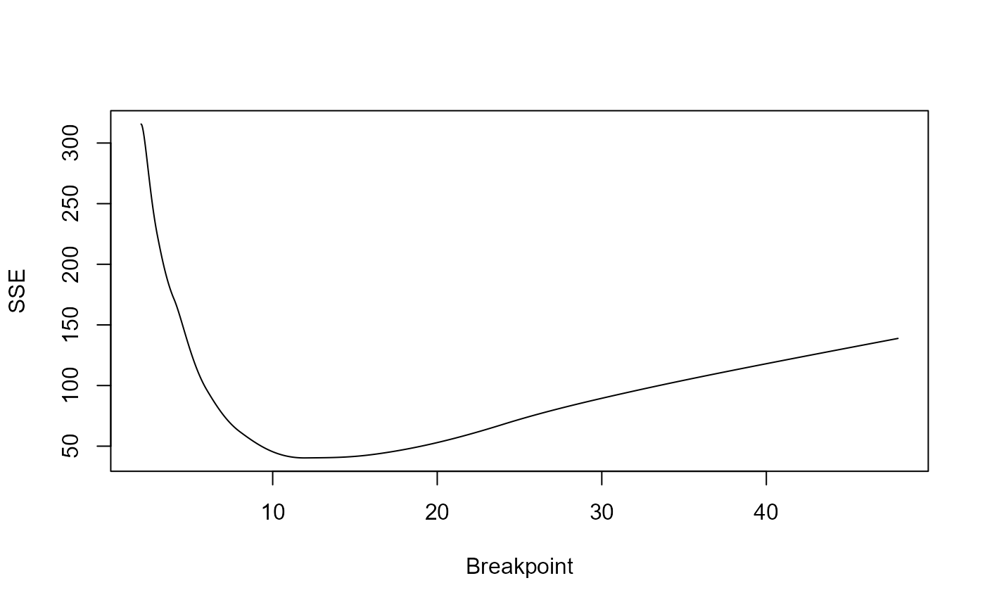
A "qrp_fit" (single series) or "qrp_multi" (per trial). The fit also carries local_minima (competing basins with their SSE excess over the optimum and a competing flag, or NULL), local_min_tol, sse_profile, compat when start was given, and bootstrap when bootstrap = TRUE (a list with ci, se, p_value, statistic, replicates, n_valid, conf_level and null_model). Because the quadratic-plateau joins smoothly, this profile is typically a single basin, unlike the stepped profile of fit_lrp().

Two ways to call

Vectors: fit_qrp(x, cv) returns a "qrp_fit".
Data frame: fit_qrp(.data, x = "x", cv = "cv", trial = "trial"); with trial, one model per trial is fit and a "qrp_multi" object is returned. Column names default to "x", "cv", "trial".

Uncertainty of the breakpoint

bootstrap = TRUE resamples the shapes (the rows of the CV table) with replacement, refits on each resample, and returns a percentile interval for $X_o$ in $bootstrap$ci, together with a bootstrap standard error.

It also tests whether the plateau is warranted. The null here is not the one used by fit_lrp(): a quadratic-plateau that never plateaus is simply a quadratic, so the null model is the unconstrained quadratic fitted on every observation, and the p-value is the proportion of null resamples whose SSE reduction matches or exceeds the observed one. A large p-value means the plateau segment buys nothing over a plain quadratic, and $X_o$ should not be read as an optimal plot size.

Set the random seed before calling to make the result reproducible.

Examples

## CV per plot shape from the bundled simulated uniformity trial
## (see ?uniformity_trial).
grid1 <- as.matrix(uniformity_trial[uniformity_trial$trial == "T1",
                                    grep("^col", names(uniformity_trial))])
cv_tab <- calc_cv_shapes(list(T1 = grid1))
#> CV by shape for 1 trial(s).
X   <- cv_tab$x
CV1 <- cv_tab$cv

## A coarse grid runs fast; the default step = 0.001 refines the third decimal
fit <- fit_qrp(X, CV1, step = 0.01)
fit
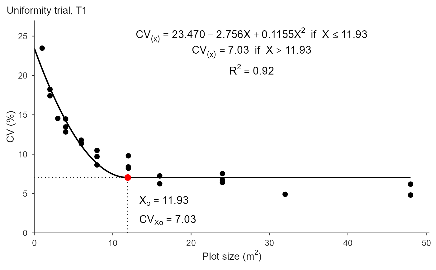
#> Quadratic Response Plateau (QRP) fit
#> Breakpoint (Xo):         11.930 
#> CV at breakpoint:        7.031 
#> R2: 0.918  R2 adj: 0.910  RMSE: 1.324  MAE: 1.069 

## The quadratic joins its plateau smoothly, so the optimum is larger than
## the one the broken-line model gives on the same data
coef(fit)
#>          a          b          c 
#> 23.4695666 -2.7557723  0.1154976 
predict(fit, newx = c(2, 5, 7.5, 15))
#> [1] 18.420012 12.578145  9.298013  7.031385

# \donttest{
## Full precision is the default; it costs about eight times more time and
## only refines the third decimal, so it is shown here rather than used
## throughout:
# fit_qrp(X, CV1)$parameters["Breakpoint"]

plot(fit, title = "Uniformity trial, T1")


## The smooth join makes the SSE profile a single basin, unlike the stepped
## profile of fit_lrp(): competing minima are rare and much worse.
plot(fit$sse_profile, type = "l", xlab = "Breakpoint", ylab = "SSE")

fit$local_minima
#> NULL

## Uncertainty of Xo, off by default. The p-value asks whether the plateau
## buys anything over a plain quadratic.
set.seed(1)
unc <- fit_qrp(X, CV1, step = 0.01, bootstrap = TRUE, n_boot = 200)
unc
#> Quadratic Response Plateau (QRP) fit
#> Breakpoint (Xo):         11.930 
#>   95% CI (percentile):  [9.885, 22.962]   SE 3.914
#>   plateau vs quadratic:  p = 0.0050  (200 resamples)
#> CV at breakpoint:        7.031 
#> R2: 0.918  R2 adj: 0.910  RMSE: 1.324  MAE: 1.069 
unc$bootstrap$ci
#> [1]  9.88500 22.96225

## Restrict the breakpoint search
fit_qrp(X, CV1, step = 0.01, search_range = c(5, 15))$parameters["Breakpoint"]
#> Breakpoint 
#>      11.93 

## One model per trial, with a summary table
trials <- rbind(
  data.frame(x = X, cv = CV1,        trial = "T1"),
  data.frame(x = X, cv = CV1 * 0.85, trial = "T2")
)
fit_qrp(trials, x = "x", cv = "cv", trial = "trial", step = 0.01)$summary
#> Using x = 'x', cv = 'cv', trial = 'trial' -> 2 trials.
#>   trial       a       b      c breakpoint plateau     R2   RMSE    AIC    BIC
#> 1    T1 23.4696 -2.7558 0.1155      11.93  7.0314 0.9178 1.3237 86.172 90.714
#> 2    T2 19.9491 -2.3424 0.0982      11.93  5.9767 0.9178 1.1252 78.696 83.238
#>   n_local
#> 1       0
#> 2       0
# }