Modified Maximum Curvature (MCM) • trialSizing

library(trialSizing)

Theory

The two plateau models cut the CV curve into pieces. The Modified Maximum Curvature method takes a different route: it fits a single smooth curve and then asks where that curve bends the most.

The relationship between CV and plot size is described by a power function,

$CV_{(X)} = \frac{a}{X^{b}} + \varepsilon = a X^{-b} + \varepsilon$

with $a > 0$ and $b > 0$ , so the CV decreases as plots grow. This curve never becomes exactly flat, which is why the method cannot simply read off a plateau. Instead it uses the curvature of the line at each point,

$K = \frac{y''}{\left(1 + y'^2\right)^{3/2}}$

and takes the optimal plot size as the point of maximum curvature, the “elbow” where the steep initial drop turns into the slow tail. Solving $\mathrm{d}K/\mathrm{d}X = 0$ for $y = aX^{-b}$ gives a closed form:

$X_o = \left[\frac{a^{2} b^{2} (2b + 1)}{b + 2}\right]^{\frac{1}{2b + 2}}, \qquad CV_{Xo} = a X_o^{-b}$

Because it locates an elbow rather than a plateau, the MCM systematically returns a smaller optimum than the LRP and QRP, and correspondingly a higher CV at the optimum. This is expected, not an error.

A note on the word “modified”: in the original paper it refers to correcting $X_c$ by the cost factors $K_1$ and $K_2$ (labour per plot and per unit area). Modern Brazilian plot-size studies drop that cost step, and fit_mcm() follows them: $X_o$ is returned in the units of x.

Two ways to estimate a and b

This is the one place in the package where the two reference articles genuinely disagree, so both are available.

method = "loglinear" is the classic route. Taking logs linearizes the model,

$\log CV_{(X)} = \log a - b \log X + \varepsilon$

so a and b come from a straight-line regression. Meier & Lessman weight that regression by the degrees of freedom of each point, following Federer (1955): CVs from large plots are computed from fewer plots and are less reliable, so they should count less. Pass df to enable that weighting.

method = "nls" (the default) fits $CV = aX^{-b}$ directly on the original scale by nonlinear least squares, seeded from the log-log fit. This is what the modern articles do, and it is consistent with fit_lrp() and fit_qrp(). If nls() fails to converge, the function falls back to the log-linear estimate with a warning rather than erroring out.

The two give visibly different answers, so choose deliberately: match whichever article you are comparing against.

References

Original method: Meier, V. D. & Lessman, K. J. (1971). Estimation of optimum field plot shape and size for testing yield in Crambe abyssinica Hochst. Crop Science, 11(5), 648-650. (After Lessman & Atkins, 1963.)

Weighting: Federer, W. T. (1955). Experimental Design. Macmillan, New York.

The implementation is validated against published results in the package tests; see Cargnelutti Filho, A., Loro, M. V., Ortiz, V. M. & Andretta, J. A. (2025). Determinação do tamanho de parcela para avaliar a massa de parte aérea de grão-de-bico. Revista Vivências, 21(43), 499-513.

Data

The bundled simulated uniformity trial (?uniformity_trial) again. n is the number of plots of each size, returned by calc_cv_shapes(), and supplies the degrees of freedom for the optional weighting.

grid_mat <- function(t)
  as.matrix(uniformity_trial[uniformity_trial$trial == t,
                             grep("^col", names(uniformity_trial))])

tab1 <- calc_cv_shapes(grid_mat("T1"))
X   <- tab1$x
n   <- tab1$n
CV1 <- tab1$cv
CV2 <- calc_cv_shapes(grid_mat("T2"))$cv
CV3 <- calc_cv_shapes(grid_mat("T3"))$cv

Both x and cv must be strictly positive: the log-log fit and the starting values are undefined otherwise.

Basic use

fit <- fit_mcm(x = X, cv = CV1)
fit
#> Modified Maximum Curvature (MCM) fit
#> Method:                  nls 
#> Weighted by df:          FALSE 
#> Breakpoint (Xo):         4.495 
#> CV at breakpoint:        12.742 
#> R2: 0.975  RMSE: 0.725

$X_o \approx 4.5$ m² with $CV_{Xo} \approx 12.7\%$ for trial 1 – as expected, well below the LRP’s ~9.2 m². The MCM is the most conservative of the three methods.

summary(fit)
#> Model coefficients (CV = a * X^(-b)):
#>          a          b 
#> 23.4700048  0.4064403 
#> 
#> Goodness of fit:
#>          Breakpoint Breakpoint_Response                  R2                RMSE 
#>           4.4948651          12.7415655           0.9753420           0.7248675

The closed form can be verified straight from the coefficients:

a <- unname(fit$coefficients["a"]); b <- unname(fit$coefficients["b"])
c(formula  = ((a^2 * b^2 * (2 * b + 1)) / (b + 2))^(1 / (2 * b + 2)),
  reported = unname(fit$parameters["Breakpoint"]))
#>  formula reported 
#> 4.494865 4.494865

predict(fit, newx = c(1, 6, 18))
#> [1] 23.470005 11.330292  7.249696

Note there is no AIC or BIC here. The MCM is not nested with the plateau models and, under "loglinear", is not even fitted on the same scale, so an information criterion would not be comparable. Compare methods on R2 and RMSE, both reported on the original scale.

Choosing the estimator

rbind(
  nls        = fit_mcm(X, CV1, method = "nls")$parameters[c("Breakpoint", "R2")],
  loglinear  = fit_mcm(X, CV1, method = "loglinear")$parameters[c("Breakpoint", "R2")],
  loglin_df  = fit_mcm(X, CV1, method = "loglinear",
                       df = n - 1)$parameters[c("Breakpoint", "R2")]
)
#>           Breakpoint        R2
#> nls         4.494865 0.9753420
#> loglinear   4.389611 0.9744473
#> loglin_df   4.525946 0.9751706

The differences are modest here but real, and they grow when the CVs of the large plots are noisy, which is exactly the case the weighting is meant to handle. The df weighting only applies with method = "loglinear"; df = NULL (the default) is the unweighted fit.

Plot

The figure has no flat segment: the power curve keeps descending, and the dotted guides mark the maximum-curvature point.

plot(fit, title = "Trial 1")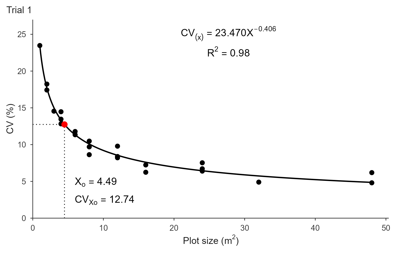

plot(fit, title = "Ensaio 1", decimal_mark = ",")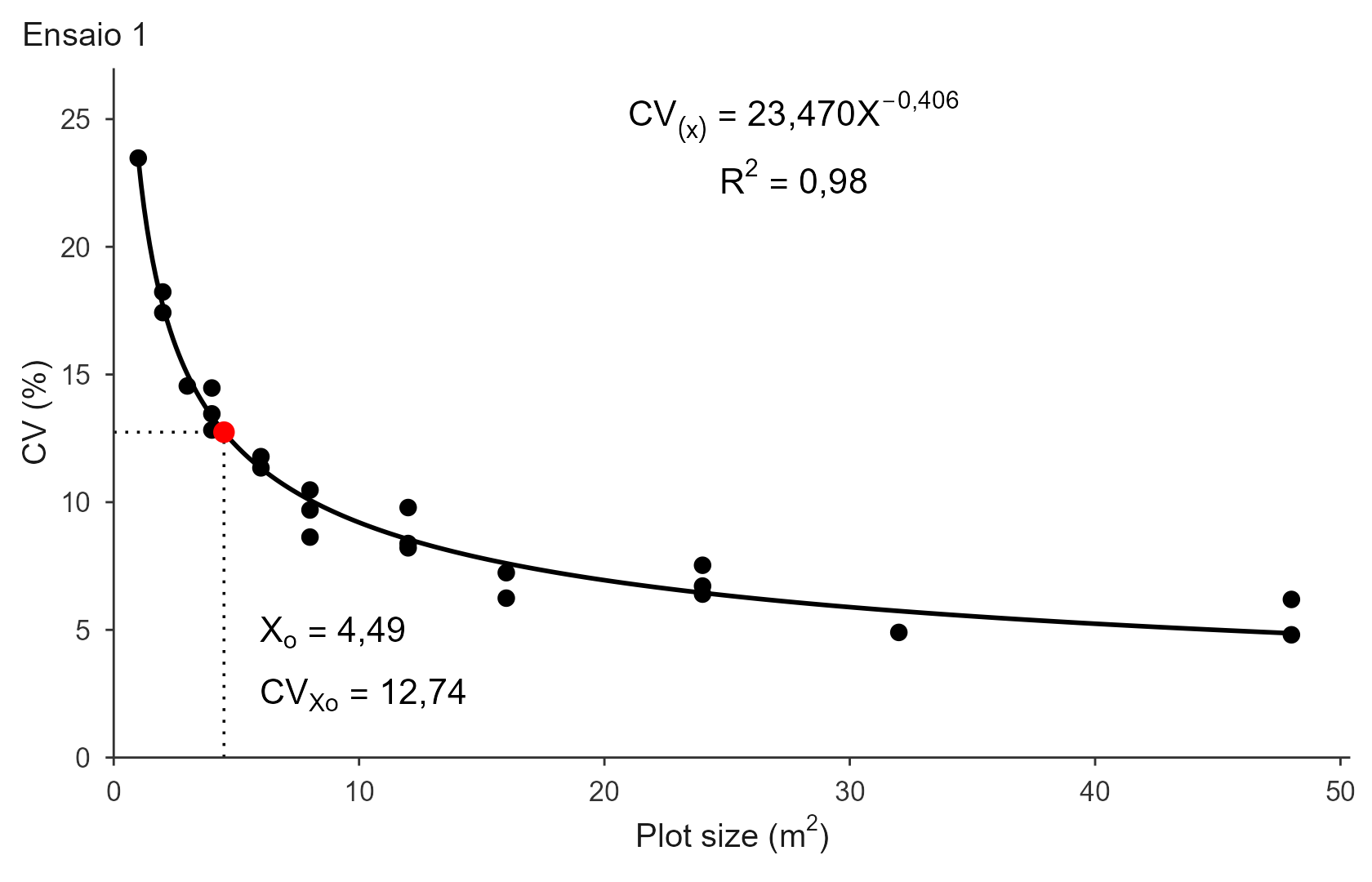

There is no cond_word argument, since the annotation has no conditional clause: a single power equation and $R^2$ , plus $X_o$ and $CV_{Xo}$ by the breakpoint.

plot(fit, title = "Trial 1",
     save = TRUE, file = "trial1_mcm.tiff", format = "tiff", dpi = 300)

Several trials at once

trials <- rbind(
  data.frame(x = X, cv = CV1, trial = "Trial 1"),
  data.frame(x = X, cv = CV2, trial = "Trial 2"),
  data.frame(x = X, cv = CV3, trial = "Trial 3")
)

res <- fit_mcm(trials, x = "x", cv = "cv", trial = "trial")
#> Using x = 'x', cv = 'cv', trial = 'trial' -> 3 trials.
res
#> MCM fits for 3 trials
#> 
#>    trial       a      b breakpoint plateau     R2   RMSE method weighted
#>  Trial 1 23.4700 0.4064     4.4949 12.7416 0.9753 0.7249    nls    FALSE
#>  Trial 2 24.9856 0.4829     4.9563 11.5337 0.8821 1.9801    nls    FALSE
#>  Trial 3 25.1900 0.4554     4.9050 12.2104 0.9068 1.6560    nls    FALSE

The three MCM breakpoints cluster below 5 m²; their mean is the overall recommendation, and all three sit well under the LRP and QRP optima.

The degrees of freedom can be supplied as a column, applied to every trial:

trials$df <- rep(n - 1, 3)
fit_mcm(trials, x = "x", cv = "cv", df = "df", trial = "trial",
        method = "loglinear")

plot(res, label_size = 3)

Warnings worth heeding

b <= 0: the CV is not decreasing with plot size, so a maximum-curvature point is meaningless for these data.
nls fallback: if the message says the fit fell back to the log-linear estimate, the reported values come from "loglinear", not "nls". The method field of the object records what was actually used.

Where to go next

vignette("lrp") and vignette("qrp") cover the plateau models, which use the same inputs and give larger optima. vignette("paranaiba") estimates the plot size straight from the raw grid instead of from CV values, and vignette("replicates") turns $CV_{Xo}$ into a number of replications.