Number of replications • trialSizing

library(trialSizing)

Theory

Choosing the plot size settles one half of the design; the other half is how many times to replicate it. The two are linked: the plot size determines the experimental precision, expressed as $CV_{Xo}$ , and that precision determines how many replications are needed to detect a given difference between treatment means.

The starting point is the least significant difference of the Tukey test, expressed as a percentage of the experiment mean:

$d = \frac{q_{\alpha(i;\,GLE)} \sqrt{QME / r}}{m} \times 100$

where $q_{\alpha(i;GLE)}$ is the Tukey critical value for $i$ treatments and $GLE$ error degrees of freedom, $QME$ is the error mean square, $r$ is the number of replications and $m$ the mean. Substituting the experimental coefficient of variation, $CV = 100\sqrt{QME}/m$ , and solving for $r$ :

$r = \left(\frac{q_{\alpha(i;\,GLE)} \cdot CV}{d}\right)^{2}$

with error degrees of freedom

$GLE = i\,(r - 1) \ \text{ for CRD}, \qquad GLE = (i - 1)(r - 1) \ \text{ for RCBD}$

Here $CV$ is $CV_{Xo}$ : the CV expected once the experiment uses the optimal plot size.

Why this needs iteration

The expression is circular. The critical value $q_\alpha$ depends on the error degrees of freedom, which depend on $r$ , which is what we are solving for. So $r$ is obtained iteratively: guess $r$ , compute $GLE$ and $q_\alpha$ , get a new $r$ , repeat until it stops moving.

calc_replicates() runs that fixed point and reports two readings of the result:

r_continuous: the converged value, e.g. 10.46. This is what the published tables print, and what to quote when comparing with an article.
r_optimal: the practical integer, ceiling(r_continuous), floored at 2. You cannot run 10.46 replications, and no design runs fewer than 2.

Smaller $d$ means finer resolution, and the cost is steep: because $r$ grows with the square of $1/d$ , halving the difference you want to detect roughly quadruples the replications needed.

References

Method: Cargnelutti Filho, A., Alves, B. M., Toebe, M., Burin, C., Santos, G. O., Facco, G., Neu, I. M. M. & Stefanello, R. B. (2014). Tamanho de parcela e número de repetições em aveia preta. Ciência Rural, 44(10), 1732-1739.

The examples below reproduce Tables 2 (CRD) and 3 (RCBD) of that article, which use black oat with $X_o = 4.14$ m² and $CV_{Xo} = 9.25\%$ .

Basic use

reps <- calc_replicates(
  treatments  = c(3, 10, 50),
  cv_percent  = 9.25,
  lsd_percent = c(10, 20, 30),
  design      = "CRD"
)
reps
#> Optimal number of replications
#> Design: CRD  CV: 9.25%  alpha: 0.05 
#> Rows: 9  | Non-converged: 0 
#> 
#>  Treatments CV_percent LSD_percent Alpha Design r_continuous r_optimal df_error
#>           3       9.25          10  0.05    CRD        10.46        11       30
#>          10       9.25          10  0.05    CRD        17.60        18      170
#>          50       9.25          10  0.05    CRD        27.41        28     1350
#>           3       9.25          20  0.05    CRD         3.56         4        9
#>          10       9.25          20  0.05    CRD         4.82         5       40
#>          50       9.25          20  0.05    CRD         6.97         7      300
#>  q_tukey converged at_floor
#>    3.486      TRUE    FALSE
#>    4.534      TRUE    FALSE
#>    5.660      TRUE    FALSE
#>    3.948      TRUE    FALSE
#>    4.735      TRUE    FALSE
#>    5.709      TRUE    FALSE

Reading the first row: with 3 treatments and a CV of 9.25%, detecting a difference of 10% of the mean needs 10.46 replications in theory, so 11 in practice. The published table gives 10.46 for that cell.

summary(reps)
#> Optimal replications (integer) by LSD (%):
#>   LSD_percent r_optimal.min r_optimal.max
#> 1          10            11            28
#> 2          20             4             7
#> 3          30             3             4

The full grid is in $data, one row per treatments × LSD combination:

head(reps$data[, c("Treatments", "LSD_percent", "r_continuous",
                   "r_optimal", "df_error", "q_tukey")])
#>   Treatments LSD_percent r_continuous r_optimal df_error  q_tukey
#> 1          3          10    10.461338        11       30 3.486420
#> 2         10          10    17.602589        18      170 4.534275
#> 3         50          10    27.412939        28     1350 5.659947
#> 4          3          20     3.556788         4        9 3.948492
#> 5         10          20     4.820311         5       40 4.734513
#> 6         50          20     6.971561         7      300 5.708613

Design, significance level

Randomized complete blocks need slightly more replications than a completely randomized design at the same precision, because blocking costs error degrees of freedom. The gap narrows as the number of treatments grows:

rbind(
  CRD  = calc_replicates(c(3, 50), 9.25, 10, design = "CRD")$data$r_continuous,
  RCBD = calc_replicates(c(3, 50), 9.25, 10, design = "RCBD")$data$r_continuous
)
#>          [,1]     [,2]
#> CRD  10.46134 27.41294
#> RCBD 10.96024 27.41574

With 3 treatments the difference is 10.46 against 10.95; with 50 it has practically vanished. Both match the published tables.

A stricter significance level raises the critical value and therefore the replications:

rbind(
  `alpha = 0.05` = calc_replicates(10, 9.25, 20, alpha = 0.05)$data$r_continuous,
  `alpha = 0.01` = calc_replicates(10, 9.25, 20, alpha = 0.01)$data$r_continuous
)
#>                  [,1]
#> alpha = 0.05 4.820311
#> alpha = 0.01 6.420760

The full workflow

In practice $CV_{Xo}$ comes from one of the plot-size methods rather than being typed in. Fitting the bundled simulated trial (?uniformity_trial) and feeding the result straight through:

grid1 <- as.matrix(uniformity_trial[uniformity_trial$trial == "T1",
                                    grep("^col", names(uniformity_trial))])
cv_tab <- calc_cv_shapes(grid1)

lrp  <- fit_lrp(cv_tab, x = "x", cv = "cv", step = 0.01)
cvxo <- unname(lrp$parameters["Breakpoint_Response"])
cvxo
#> [1] 6.944847

calc_replicates(treatments = c(5, 10, 20), cv_percent = cvxo,
                lsd_percent = c(10, 20), design = "RCBD")$data[
                  , c("Treatments", "LSD_percent", "r_continuous", "r_optimal")]
#>   Treatments LSD_percent r_continuous r_optimal
#> 1          5          10     8.163305         9
#> 2         10          10    10.198463        11
#> 3         20          10    12.420940        13
#> 4          5          20     2.929867         3
#> 5         10          20     3.073030         4
#> 6         20          20     3.404826         4

So a trial designed with plots of about 9 m² would carry an expected CV near 7%, and the table reads off how many replications are needed to detect a given difference between treatment means.

Plot

Over a range of treatments the trade-off becomes visual: one line per LSD level, showing how the requirement climbs as the number of treatments grows and as the target difference tightens.

reps <- calc_replicates(treatments = 3:50, cv_percent = 9.25,
                        lsd_percent = c(10, 20, 30), design = "CRD")

plot(reps, title = "Replications needed (black oat)")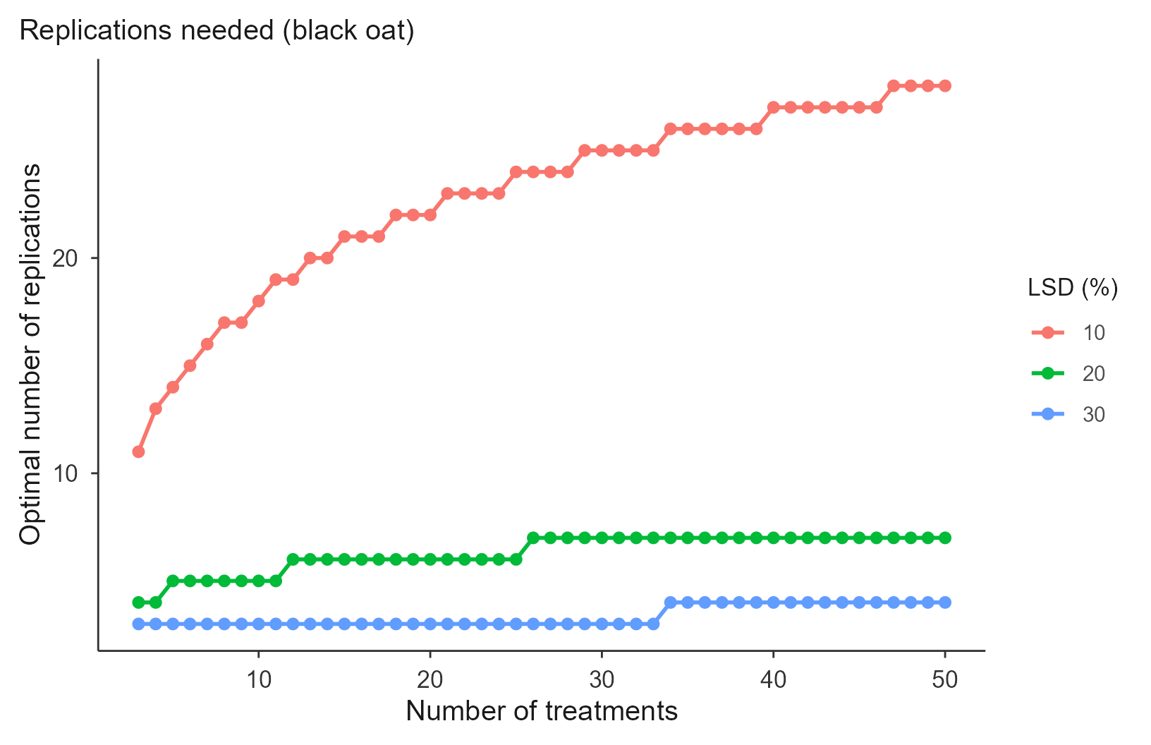

The default plots the integer r_optimal, which is why the lines are stepped. For the smooth theoretical curve, plot the continuous value:

plot(reps, y_var = "r_continuous", title = "Replications (continuous)")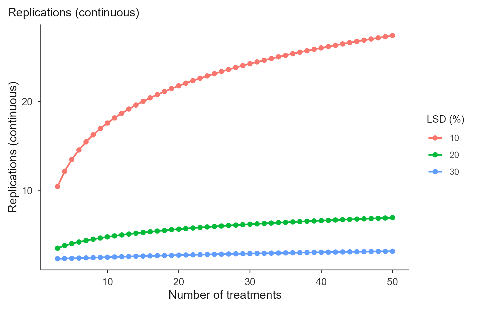

plot(reps, title = "Replications needed",
     save = TRUE, file = "replications.tiff", format = "tiff", dpi = 300)

Reading the results

The article’s conclusion illustrates how these numbers are used in practice. With a CV of 9.25%, detecting differences of 10% of the mean would need around 27 replications for 50 treatments, which is not feasible in the field. Turning the question around and fixing $r = 4$ , a common choice in the literature, the detectable difference becomes about 26.7% of the mean. That is the honest statement of what the experiment can and cannot resolve.

The function does not pick a precision for you, and it should not: that decision depends on how large a difference matters agronomically and how much field area is available. What it does is make the trade-off explicit before the experiment is installed rather than after.

Where to go next

vignette("lrp"), vignette("qrp") and vignette("mcm") cover the CV-based plot-size methods that supply $CV_{Xo}$ ; vignette("paranaiba") derives it directly from the raw trial grid.