Linear Response Plateau (LRP) • trialSizing

library(trialSizing)

Theory

In a uniformity trial, adjacent basic experimental units (BEU) are grouped into plots of increasing size X, and the coefficient of variation CV(X) is computed among plots of each size. The CV falls as plots get larger, but the gain shrinks: past a certain size, extra area buys almost no precision. The Linear Response Plateau model formalizes that as two joined straight lines,

$CV_{(X)} = \begin{cases} a + bX + \varepsilon, & \text{if } X \le X_o \\ p + \varepsilon, & \text{if } X > X_o \end{cases}$

The first segment falls with slope $b < 0$ ; the second is flat at the plateau $p$ . The join between them is the estimate of interest: $X_o$ is the optimal plot size and $p = CV_{Xo}$ is the CV expected at that size. From the model,

$X_o = \frac{p - a}{b}, \qquad CV_{Xo} = a + b X_o$

How the breakpoint is estimated

Fitting a broken line is awkward for general-purpose nonlinear least squares. The model has a kink, and the residual sum of squares (SSE) is a stepped function of the breakpoint: moving $X_o$ between two observed plot sizes does not change which points fall in each segment, so the SSE stays flat and its derivative is zero. Gradient-based fitters such as nls() and nlsLM() stall on those flat steps and return whichever basin their starting value happened to land in.

fit_lrp() avoids this by profiling the breakpoint. It walks a fine grid of candidate values for $X_o$ ; at each candidate the model becomes linear, so the coefficients come from ordinary least squares. The candidate with the smallest SSE wins. There are no starting values and no convergence failures, and the result is the global least-squares optimum by construction.

That does not make the breakpoint unambiguous, though: the profile may have several basins that fit almost equally well. See Competing breakpoints below.

References

Original method: Paranaíba, P. F., Ferreira, D. F. & Morais, A. R. (2009). Tamanho ótimo de parcelas experimentais: proposição de métodos de estimação. Revista Brasileira de Biometria, 27(2), 255-268.

The implementation is validated against published results in the package tests; see Cargnelutti Filho, A., Loro, M. V., Ortiz, V. M. & Andretta, J. A. (2025). Determinação do tamanho de parcela para avaliar a massa de parte aérea de grão-de-bico. Revista Vivências, 21(43), 499-513.

Data

The examples use the bundled simulated uniformity trial (?uniformity_trial): an 8 × 12 grid of 1 m² BEU per trial, grouped by calc_cv_shapes() into plot shapes. X is the plot size in BEU and CV1–CV3 are the CVs of trials 1 to 3.

grid_mat <- function(t)
  as.matrix(uniformity_trial[uniformity_trial$trial == t,
                             grep("^col", names(uniformity_trial))])

tab1 <- calc_cv_shapes(grid_mat("T1"))
X   <- tab1$x
CV1 <- tab1$cv
CV2 <- calc_cv_shapes(grid_mat("T2"))$cv
CV3 <- calc_cv_shapes(grid_mat("T3"))$cv

Note that X repeats: several shapes share the same size (four different shapes of 6 BEU, for instance). Supply one CV per shape, never the mean per size, or the fit loses the within-size variability it needs.

Basic use

Every fit below passes step = 0.01 rather than the default 0.001. That is only to keep this vignette quick to build, and to keep every number on this page consistent with the others: the coarser grid already resolves $X_o$ to two decimals, and only the third decimal differs. See Fine-tuning for what step does.

fit <- fit_lrp(x = X, cv = CV1, step = 0.01)
fit
#> Linear Response Plateau (LRP) fit
#> Method:                  segment  
#> Breakpoint (Xo):         9.160 
#> CV at breakpoint:        6.945 
#> R2: 0.893  RMSE: 1.513  AIC: 92.3  BIC: 96.9 
#> 
#> Local minima of the SSE profile (8):
#>   Xo =   7.400   SSE  +15.3% vs optimum
#>   Xo =  12.820   SSE  +34.5% vs optimum
#>   Xo =   5.750   SSE  +50.1% vs optimum
#>   ... see $local_minima for all

$X_o \approx 9.2$ m² with $CV_{Xo} \approx 6.9\%$ for trial 1. The competing minima listed underneath are explained further down.

summary() splits the model coefficients from the fit statistics:

summary(fit)
#> Model coefficients:
#>         a         b 
#> 21.049460 -1.539805 
#> 
#> Goodness of fit:
#>          Breakpoint Breakpoint_Response                  R2                RMSE 
#>           9.1600000           6.9448467           0.8925663           1.5130369 
#>                 AIC                 BIC 
#>          92.3206384          96.8626153

Everything is also available directly:

fit$coefficients
#>         a         b 
#> 21.049460 -1.539805
fit$parameters["Breakpoint"]
#> Breakpoint 
#>       9.16
round(fit$residuals[1:5], 3)
#> [1]  3.964  0.262 -0.545 -1.879 -0.419

predict() evaluates the fitted model at any plot size, which is handy to check the plateau behaviour:

predict(fit, newx = c(1, 5, 12, 15))
#> [1] 19.509655 13.350435  6.944847  6.944847

The last two values are identical: past the breakpoint the model is flat.

Plot

The plot() method draws the article-style figure. Title and styling go here, not in fit_lrp():

plot(fit, title = "Trial 1")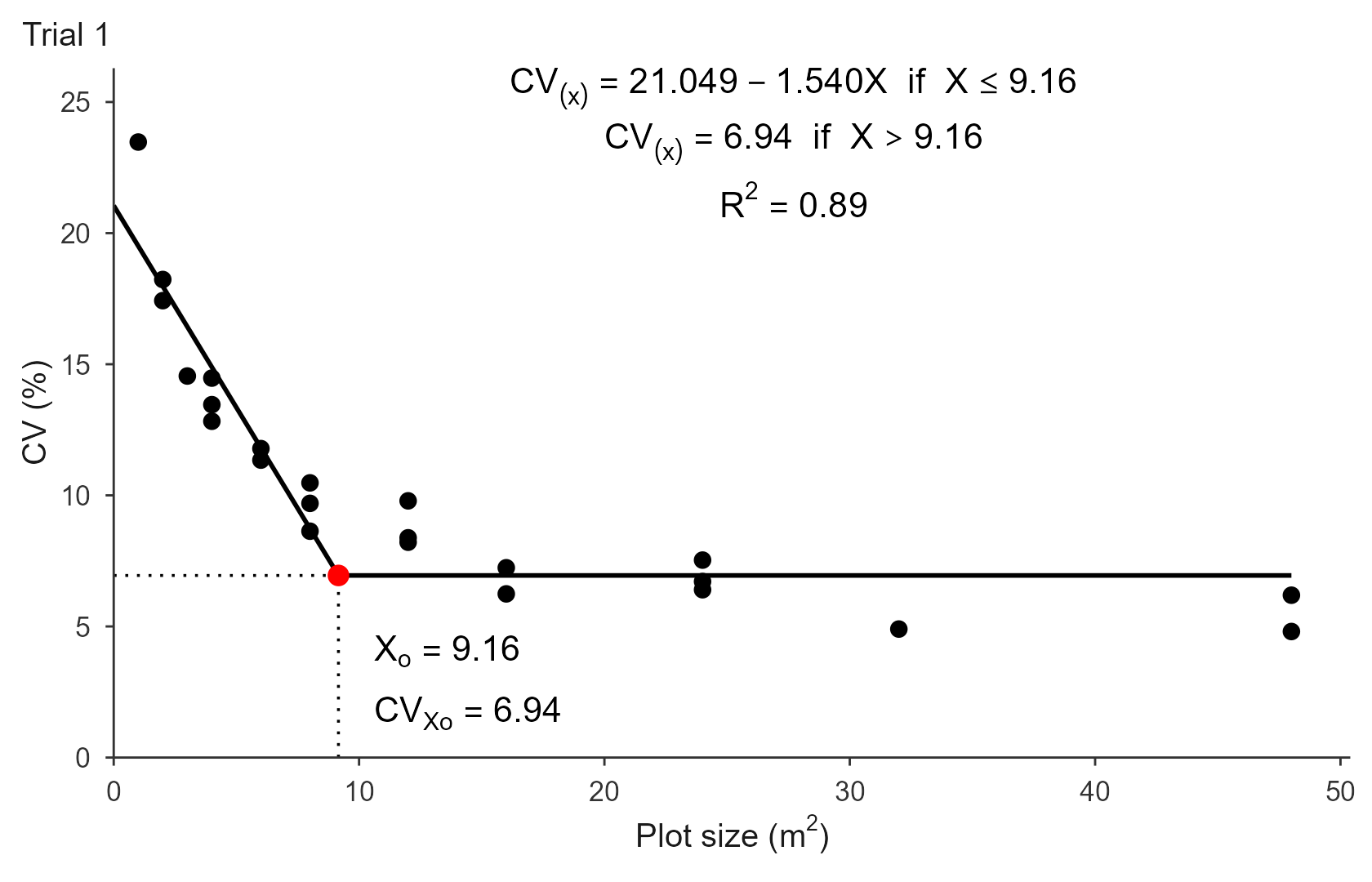

For Portuguese-language figures, switch the decimal mark and the conditional word:

plot(fit, title = "Ensaio 1", decimal_mark = ",", cond_word = "se")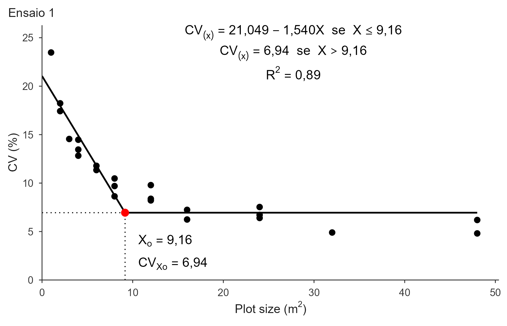

Other useful arguments: annotate_model = FALSE drops the equation block, base_size / label_size / title_size scale the text, theme accepts any ggplot2 theme, and xlab / ylab relabel the axes.

To export, set save = TRUE. TIFF is written with LZW compression; PDF and EPS are vector formats, usually the better choice for line art like this.

plot(fit, title = "Trial 1",
     save = TRUE, file = "trial1.tiff", format = "tiff",
     dpi = 300, width = 18, height = 12, units = "cm")

Several trials at once

Pass a data frame plus the column names. One model is fitted per trial:

trials <- rbind(
  data.frame(x = X, cv = CV1, trial = "Trial 1"),
  data.frame(x = X, cv = CV2, trial = "Trial 2"),
  data.frame(x = X, cv = CV3, trial = "Trial 3")
)

res <- fit_lrp(trials, x = "x", cv = "cv", trial = "trial", step = 0.01)
#> Using x = 'x', cv = 'cv', trial = 'trial' -> 3 trials.
res$summary
#>     trial       a       b breakpoint plateau     R2   RMSE     AIC     BIC
#> 1 Trial 1 21.0495 -1.5398       9.16  6.9448 0.8926 1.5130  92.321  96.863
#> 2 Trial 2 19.3597 -1.0725      14.40  3.9162 0.8341 2.3486 112.547 117.089
#> 3 Trial 3 21.3271 -1.5075      10.11  6.0860 0.8019 2.4137 113.805 118.347
#>   n_local
#> 1       8
#> 2       7
#> 3       8

The three breakpoints differ from trial to trial, as real trials do; their mean is the natural overall recommendation. The n_local column counts competing basins per trial.

The individual fits stay accessible, so any single trial can be inspected or plotted as usual:

res$fits[["Trial 2"]]
#> Linear Response Plateau (LRP) fit
#> Method:                  segment  
#> Breakpoint (Xo):         14.400 
#> CV at breakpoint:        3.916 
#> R2: 0.834  RMSE: 2.349  AIC: 112.5  BIC: 117.1 
#> 
#> Local minima of the SSE profile (7):
#>   Xo =  17.500   SSE   +0.2% vs optimum  *
#>   Xo =  10.960   SSE  +12.4% vs optimum
#>   Xo =  24.860   SSE  +25.9% vs optimum
#>   ... see $local_minima for all
#>   * fits within 10% of the optimum (local_min_tol); breakpoint not sharply identified

plot() on the multi-trial object arranges the panels in a grid of at most six (3 rows × 2 columns), paginating into separate figures beyond that. It needs the patchwork package.

plot(res, decimal_mark = ",", cond_word = "se", label_size = 3)

Column names default to "x", "cv" and "trial", so fit_lrp(trials) alone works when the data frame already uses those names. Missing columns produce a clear error rather than a cryptic one:

fit_lrp(trials, x = "x", cv = "CV", trial = "trial")
#> Error:
#> ! Column(s) not found in `.data`: CV.
#>   Available columns: x, cv, trial.

Competing breakpoints

Uniformity trials rarely have many distinct plot sizes, so the SSE profile is stepped and often has several local minima. The grid search always returns the global optimum, but a second basin may fit nearly as well. When that happens the breakpoint is not sharply identified, and different software will legitimately report different values.

fit_lrp() makes this visible instead of hiding it. Every fit carries $local_minima, listing each basin with its SSE and its excess over the optimum. Basins fitting within local_min_tol (10% by default) are flagged in the competing column and starred by print(). Nothing is signalled by a warning: stepped profiles almost always have several minima, so a warning would fire on nearly every fit and stop meaning anything.

fit2 <- fit_lrp(X, CV2, step = 0.01)

lm2 <- fit2$local_minima
lm2[c("breakpoint", "SSE", "SSE_excess")] <-
  round(lm2[c("breakpoint", "SSE", "SSE_excess")], 3)
lm2
#>   breakpoint     SSE SSE_excess competing
#> 1      17.50 127.138      0.002      TRUE
#> 2      10.96 142.641      0.124     FALSE
#> 3      24.86 159.674      0.259     FALSE
#> 4      32.00 183.044      0.443     FALSE
#> 5       7.69 196.890      0.552     FALSE
#> 6       5.99 271.638      1.141     FALSE
#> 7       3.99 404.290      2.187     FALSE

Read the SSE_excess column as “how much worse than the optimum”. When a runner-up basin fits only a few percent worse than the reported optimum, those two plot sizes are effectively tied and the breakpoint carries more uncertainty than its decimals suggest. A competitor 30% worse, in contrast, can be safely dismissed.

The whole profile is available for inspection or plotting:

prof <- fit2$sse_profile
plot(prof$breakpoint, prof$SSE, type = "l",
     xlab = "Breakpoint", ylab = "SSE", las = 1)
abline(v = fit2$parameters["Breakpoint"], col = "forestgreen", lwd = 2)
abline(v = fit2$local_minima$breakpoint, col = "red", lty = 2)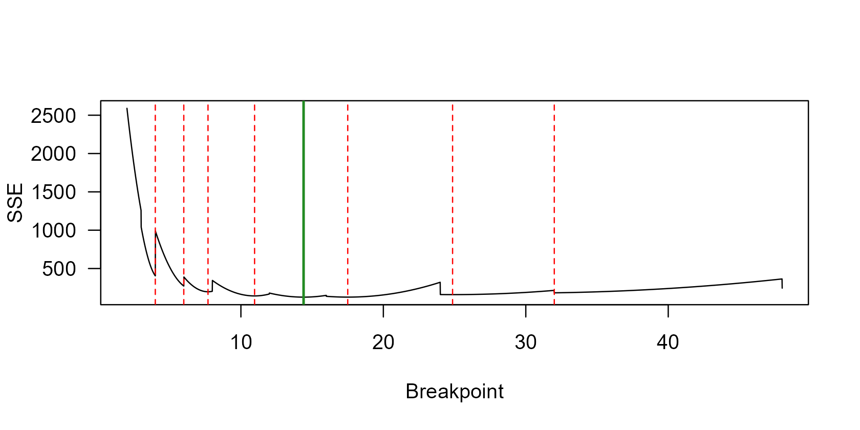

Reproducing a fit from another package

When a colleague’s nls()-based script or another package reports a different breakpoint, it is usually because their starting value landed in another basin. The start argument reproduces that solution without changing the reported fit, so you can see exactly what they got and what it cost in fit quality:

soy_x  <- c(1, 2, 4, 8, 2, 4, 8, 16, 4, 8, 16, 32, 5, 10, 20, 40)
soy_cv <- c(18.699092, 14.130115, 10.321934, 7.990773, 12.690754, 9.995547,
            7.916291, 7.588785, 9.276139, 7.130636, 4.777755, 4.279987,
            8.411412, 5.818440, 3.431264, 3.335962)

seeded <- fit_lrp(soy_x, soy_cv, start = 10.17, step = 0.01)
seeded$compat
#> $start
#> [1] 10.17
#> 
#> $breakpoint
#> [1] 10.17
#> 
#> $coefficients
#>        a        b 
#> 15.76286 -1.08947 
#> 
#> $plateau
#> [1] 4.682951
#> 
#> $SSE
#> [1] 43.17176
#> 
#> $SSE_excess
#> [1] 0.1509463

The reported fit is still the optimum at 5.79; $compat shows that a fitter seeded near 10 would stop at 10.17 with an SSE 15% higher. That is a large enough gap to prefer the optimum, but the number is there for you to judge, and to cite when reconciling results across software.

Deciding between basins

A statistically better fit is not automatically the better agronomic answer. A very early breakpoint can be a “false plateau”: the trial may lack the range of plot sizes needed for a genuine plateau to emerge, so the model latches onto a flat stretch that is really just noise. When two basins are close in SSE, weigh the number of points supporting each segment, whether the plateau looks plausible on the plot, and what plot sizes are feasible in the field.

Once you have decided, search_range documents the choice explicitly:

fit_lrp(soy_x, soy_cv, search_range = c(8, 20), step = 0.01)$parameters["Breakpoint"]
#> Breakpoint 
#>       9.54

Fine-tuning

search_range restricts where the breakpoint is searched, which helps when an outlier in the transition zone pulls the estimate somewhere implausible. It must fall inside the data range, and a warning is issued if the breakpoint lands on the edge of the range you gave.

fit_lrp(X, CV1, search_range = c(5, 12), step = 0.01)$parameters["Breakpoint"]
#> Breakpoint 
#>       9.16

step is the grid resolution, 0.001 by default. Coarser grids are faster and slightly less precise:

fit_lrp(X, CV1, step = 0.01)$parameters["Breakpoint"]
#> Breakpoint 
#>       9.16

method chooses how the linear coefficients are estimated at each candidate breakpoint. "segment" (default) uses only the observations with x <= X0, reproducing the published procedure. "ramp" uses every observation on the basis pmin(x, X0), the standard least-squares LRP; the plateau points then also inform the descending line, which can shift the optimum.

fit_lrp(X, CV1, method = "ramp", step = 0.01)$parameters["Breakpoint"]
#> Breakpoint 
#>       9.16

local_min_tol sets how close a competitor must fit to be flagged as competing. It changes labelling only, never the fit: lower it (say 0.02) to mark only near-ties, raise it to mark any competitor.

fit_lrp(X, CV2, local_min_tol = 0.02, step = 0.01)$local_minima$competing
#> [1]  TRUE FALSE FALSE FALSE FALSE FALSE FALSE

Warnings worth heeding

Two situations trigger a warning, and both mean the estimate deserves a second look rather than direct use:

Non-negative slope: the CV is not decreasing with plot size, so the “descent then plateau” reading does not hold for these data.
Breakpoint at the edge of the search range: the trial may not span enough plot sizes to bracket the true optimum, so the CV may still be falling at the largest size evaluated.

A third situation is reported without a warning, because it is too common for one to be informative: a competing local minimum, where another breakpoint fits nearly as well and the estimate is not sharply identified. Check the competing column of $local_minima before reporting a single value.

Where to go next

vignette("qrp") and vignette("mcm") cover the other two CV-based methods, which take the same inputs and usually give a larger and a smaller optimum respectively. The QRP joins its plateau smoothly, so its SSE profile is a single smooth basin and competing minima are rare. vignette("replicates") shows how $CV_{Xo}$ feeds into the number of replications.