Quadratic Response Plateau (QRP) • trialSizing

library(trialSizing)

Theory

The Quadratic Response Plateau model answers the same question as the LRP, but replaces the straight descent with a curve:

$CV_{(X)} = \begin{cases} a + bX + cX^2 + \varepsilon, & \text{if } X \le X_o \\ p + \varepsilon, & \text{if } X > X_o \end{cases}$

The plateau starts where the parabola reaches its vertex, so the two pieces meet smoothly (no kink, unlike the LRP). That gives closed forms for both quantities of interest:

$X_o = -\frac{b}{2c}, \qquad CV_{Xo} = p = a - \frac{b^2}{4c}$

For the curve to descend and then flatten, $b < 0$ and $c > 0$ .

Because the descent is curved rather than straight, the QRP stays above a straight line for longer and reaches its plateau later. In practice this means QRP almost always gives a larger optimum than LRP, which in turn gives a larger one than the MCM. That ordering (MCM < LRP < QRP) is reported across many crops and is not a defect of any of the methods: they answer the same question with different assumptions about the shape of the decay.

How the breakpoint is estimated

The published implementations fit this model with nls() or nlsLM() and fixed starting values. That is fragile: the starting values are not derived from the data, and a failure to converge can pass silently.

fit_qrp() uses the same grid-search strategy as fit_lrp(). Once $X_o$ is fixed, the model can be written as

$CV_{(X)} = A + c\,(X - X_o)^2 \ \text{ for } X \le X_o, \qquad CV_{(X)} = A \ \text{ for } X > X_o$

which is linear in the plateau level $A$ and the curvature $c$ . So each candidate breakpoint is fitted by ordinary least squares, and the one with the smallest residual sum of squares is returned. The reported a, b, c are converted back to the usual parametrization via $a = A + cX_o^2$ and $b = -2cX_o$ . The result is numerically identical to a converged nls() fit, without the starting values.

References

Original method: Peixoto, A. P. B., Faria, G. A. & Morais, A. R. (2011). Modelos de regressão com platô na estimativa do tamanho de parcelas em experimento de conservação in vitro de maracujazeiro. Ciência Rural, 41(11), 1907-1913.

The implementation is validated against published results in the package tests; see Cargnelutti Filho, A., Loro, M. V., Ortiz, V. M. & Andretta, J. A. (2025). Determinação do tamanho de parcela para avaliar a massa de parte aérea de grão-de-bico. Revista Vivências, 21(43), 499-513.

Data

The bundled simulated uniformity trial (?uniformity_trial), the same data used throughout the package.

grid_mat <- function(t)
  as.matrix(uniformity_trial[uniformity_trial$trial == t,
                             grep("^col", names(uniformity_trial))])

tab1 <- calc_cv_shapes(grid_mat("T1"))
X   <- tab1$x
CV1 <- tab1$cv
CV2 <- calc_cv_shapes(grid_mat("T2"))$cv
CV3 <- calc_cv_shapes(grid_mat("T3"))$cv

Basic use

Every fit below passes step = 0.01 rather than the default 0.001. That is only to keep this vignette quick to build, and to keep every number on this page consistent with the others: the coarser grid already resolves $X_o$ to two decimals, and only the third decimal differs. See Fine-tuning for what step does.

fit <- fit_qrp(x = X, cv = CV1, step = 0.01)
fit
#> Quadratic Response Plateau (QRP) fit
#> Breakpoint (Xo):         11.930 
#> CV at breakpoint:        7.031 
#> R2: 0.918  R2 adj: 0.910  RMSE: 1.324  MAE: 1.069

$X_o \approx 11.9$ m² for trial 1, noticeably larger than the LRP estimate of about 9.2 m² on the same data: the smooth join always pushes the optimum out.

summary(fit)
#> Model coefficients:
#>          a          b          c 
#> 23.4695666 -2.7557723  0.1154976 
#> 
#> Goodness of fit:
#>          Breakpoint Breakpoint_Response                  R2              R2_adj 
#>          11.9300000           7.0313850           0.9177688           0.9095457 
#>                RMSE                 MAE                 AIC                 BIC 
#>           1.3237245           1.0691734          86.1718431          90.7138200 
#>                 SSE                 MSE 
#>          40.3016712           1.7522466

The QRP reports more fit statistics than the LRP: alongside R2 and RMSE it returns R2_adj (adjusted for the extra parameter), MAE, SSE and MSE.

The closed forms can be checked directly against the coefficients:

cf <- fit$coefficients
c(vertex = unname(-cf["b"] / (2 * cf["c"])),
  reported = unname(fit$parameters["Breakpoint"]))
#>   vertex reported 
#>    11.93    11.93

predict(fit, newx = c(1, 5, 11, 15))
#> [1] 20.829292 12.578145  7.131279  7.031385

Plot

The figure follows the same layout as the LRP, with the quadratic term in the annotated equation:

plot(fit, title = "Trial 1")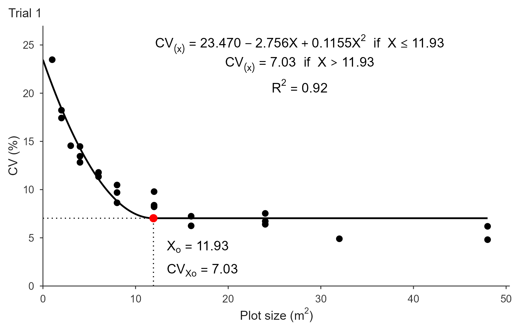

plot(fit, title = "Ensaio 1", decimal_mark = ",", cond_word = "se")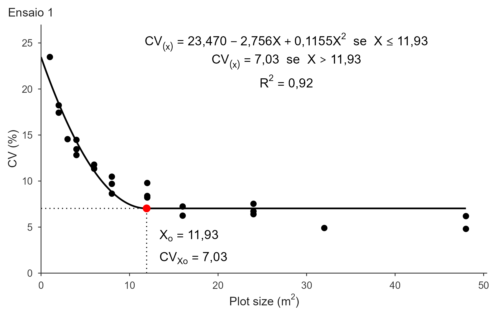

The curvature coefficient c is small, so it gets its own decimal control, digits_c (4 by default), separate from digits_coef for a and b.

plot(fit, title = "Trial 1",
     save = TRUE, file = "trial1_qrp.pdf", format = "pdf",
     width = 18, height = 12, units = "cm")

Several trials at once

The data-frame interface is identical to fit_lrp():

trials <- rbind(
  data.frame(x = X, cv = CV1, trial = "Trial 1"),
  data.frame(x = X, cv = CV2, trial = "Trial 2"),
  data.frame(x = X, cv = CV3, trial = "Trial 3")
)

res <- fit_qrp(trials, x = "x", cv = "cv", trial = "trial", step = 0.01)
#> Using x = 'x', cv = 'cv', trial = 'trial' -> 3 trials.
res
#> QRP fits for 3 trials
#> 
#>    trial       a       b      c breakpoint plateau     R2   RMSE     AIC
#>  Trial 1 23.4696 -2.7558 0.1155      11.93  7.0314 0.9178 1.3237  86.172
#>  Trial 2 20.4941 -1.5222 0.0338      22.49  3.3774 0.8666 2.1062 107.535
#>  Trial 3 23.1963 -2.4042 0.0839      14.33  5.9702 0.8298 2.2373 110.314
#>      BIC n_local
#>   90.714       0
#>  112.077       0
#>  114.856       0

The summary table carries the extra c column, since the QRP has three coefficients. The three breakpoints average 10.25 m², the article’s QRP figure.

res$fits[["Trial 3"]]
#> Quadratic Response Plateau (QRP) fit
#> Breakpoint (Xo):         14.330 
#> CV at breakpoint:        5.970 
#> R2: 0.830  R2 adj: 0.813  RMSE: 2.237  MAE: 1.660

plot(res, label_size = 3)

Fine-tuning

search_range and step behave exactly as in fit_lrp():

fit_qrp(X, CV1, search_range = c(6, 15), step = 0.01)$parameters["Breakpoint"]
#> Breakpoint 
#>      11.93
fit_qrp(X, CV1, step = 0.01)$parameters["Breakpoint"]
#> Breakpoint 
#>      11.93

There is no method argument here. The LRP has one because the published procedure fits the descending line using only the pre-breakpoint points; the QRP has no such variant.

Warnings worth heeding

Non-positive curvature (c <= 0): the parabola opens downward or is flat, so the “descend then plateau” shape does not hold for these data.
Breakpoint at the edge of the search range: the trial may not span enough plot sizes to bracket the optimum.

Comparing with the other methods

Fitting all three CV-based methods on the same trial shows the usual ordering:

data.frame(
  method = c("MCM", "LRP", "QRP"),
  Xo = c(fit_mcm(X, CV1)$parameters["Breakpoint"],
         fit_lrp(X, CV1, step = 0.01)$parameters["Breakpoint"],
         fit_qrp(X, CV1, step = 0.01)$parameters["Breakpoint"]),
  row.names = NULL
)
#>   method        Xo
#> 1    MCM  4.494865
#> 2    LRP  9.160000
#> 3    QRP 11.930000

Which one to report is a judgement call. The larger optimum is the conservative choice: it buys more precision at the cost of more field area. The validation article recommends the LRP value as its overall answer, while noting that LRP and QRP delivered statistically indistinguishable precision at the optimum.

See vignette("lrp") and vignette("mcm") for the other two methods, and vignette("replicates") for turning $CV_{Xo}$ into a number of replications.