Fit the Modified Maximum Curvature (MCM) plot-size model

Estimates the optimal plot size by the modified maximum curvature method of Meier & Lessman (1971). The relationship $CV = a\,X^{-b}$ is fit by linear regression of $\log CV$ on $\log X$, and the optimum is the point of maximum curvature $$X_c = \left[ a^2 b^2 (2b + 1) / (b + 2) \right]^{1/(2b + 2)}.$$

Usage

fit_mcm(
  .data = NULL,
  x = NULL,
  cv = NULL,
  df = NULL,
  trial = NULL,
  method = c("nls", "loglinear"),
  bootstrap = FALSE,
  n_boot = 1000,
  conf_level = 0.95
)

Arguments

.data: optional data frame; when supplied the other arguments are column names.
x, cv: numeric vectors (plot size and CV in percent), or column names.
df: optional degrees of freedom per point for the Federer (1955) weighting, as a vector or a column name. NULL = unweighted.
trial: optional column name identifying the trial.
method: estimation method: "nls" (default, original scale, as in the modern Brazilian plot-size papers) or "loglinear" (Meier & Lessman regression).
bootstrap: logical; if TRUE, also estimate the uncertainty of $X_c$ by resampling the shapes (default FALSE). See the section "Uncertainty of the optimum".
n_boot: number of bootstrap resamples (default 1000), used only when bootstrap = TRUE.
conf_level: confidence level of the percentile interval (default 0.95), used only when bootstrap = TRUE.

Value

An "mcm_fit" (single series) or "mcm_multi" (per trial). With bootstrap = TRUE the fit also carries bootstrap, a list with ci, se, ci_b, replicates, n_valid and conf_level.

Estimation method

method = "nls" (default) fits $CV = a X^{-b}$ by nonlinear least squares on the original scale (seeded from the log-log fit), reproducing Cargnelutti Filho et al. (2025) and the modern Brazilian plot-size papers. method = "loglinear" fits the line $\log CV = \log a - b \log X$ (the classic Meier & Lessman route). If "nls" fails to converge it falls back to the log-linear estimate with a warning.

Degrees-of-freedom correction

Pass df, the degrees of freedom of each point, to weight the fit as proposed by Federer (1955); this down-weights the CV of larger plot sizes, estimated from fewer plots. Some authors apply it, others do not; df = NULL (default) is unweighted. The cost-factor modification (K1, K2) of the classic method is not applied; $X_c$ is in the units of x.

Uncertainty of the optimum

bootstrap = TRUE resamples the shapes with replacement, refits, and returns a percentile interval for $X_c$ in $bootstrap$ci.

Unlike fit_lrp() and fit_qrp(), there is no test for the existence of the optimum, because there is no breakpoint whose presence is in doubt: the curve $CV = a X^{-b}$ has a point of maximum curvature whenever $b > 0$. What can be questioned is $b$. Its bootstrap interval is therefore reported as $bootstrap$ci_b; if that interval covers zero, the CV does not demonstrably fall with plot size and $X_c$ carries no meaning.

Set the random seed before calling to make the result reproducible.

Two ways to call

Vectors: fit_mcm(x, cv, df = NULL) returns an "mcm_fit".
Data frame: fit_mcm(.data, x = "x", cv = "cv", df = "df", trial = "trial"); with trial, one model per trial is fit and an "mcm_multi" object is returned.

References

Meier, V. D. & Lessman, K. J. (1971). Estimation of optimum field plot shape and size for testing yield in Crambe abyssinica Hochst. Crop Science, 11, 648-650.
Federer, W. T. (1955). Experimental Design. Macmillan, New York.

Examples

## CV per plot shape from the bundled simulated uniformity trial
## (see ?uniformity_trial).
grid1 <- as.matrix(uniformity_trial[uniformity_trial$trial == "T1",
                                    grep("^col", names(uniformity_trial))])
cv_tab <- calc_cv_shapes(list(T1 = grid1))
#> CV by shape for 1 trial(s).
X   <- cv_tab$x
CV1 <- cv_tab$cv

fit <- fit_mcm(X, CV1)
fit
#> Modified Maximum Curvature (MCM) fit
#> Method:                  nls 
#> Weighted by df:          FALSE 
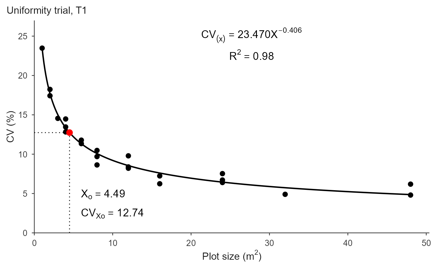
#> Breakpoint (Xo):         4.495 
#> CV at breakpoint:        12.742 
#> R2: 0.975  RMSE: 0.725 

## The fitted decay CV = a * X^-b, and the CV expected at unobserved sizes
coef(fit)
#>          a          b 
#> 23.4700048  0.4064403 
predict(fit, newx = c(2, 5, 7.5, 15))
#> [1] 17.707712 12.201791 10.347918  7.807325

## "loglinear" is the classic Meier & Lessman route (regression of log CV on
## log X); "nls" (default) fits on the original scale and is what the modern
## plot-size articles report. They rarely agree exactly.
c(nls       = unname(fit$parameters["Breakpoint"]),
  loglinear = unname(fit_mcm(X, CV1, method = "loglinear")$parameters["Breakpoint"]))
#>       nls loglinear 
#>  4.494865  4.389611 

## Federer (1955) weighting: the CV of a large plot size rests on fewer
## plots, so pass the degrees of freedom of each point (n - 1) to down-weight
## it. The plot count n is carried in the CV table.
fit_mcm(X, CV1, df = cv_tab$n - 1)$parameters["Breakpoint"]
#> Breakpoint 
#>   4.506839 

## Uncertainty of Xc, off by default. There is no existence test here: the
## curve always has a maximum-curvature point when b > 0, so what gets an
## interval is b itself.
set.seed(1)
unc <- fit_mcm(X, CV1, bootstrap = TRUE, n_boot = 200)
unc
#> Modified Maximum Curvature (MCM) fit
#> Method:                  nls 
#> Weighted by df:          FALSE 
#> Breakpoint (Xo):         4.495 
#>   95% CI (percentile):  [4.171, 4.787]   SE 0.140
#>   exponent b:            [0.373, 0.435]  (200 resamples)
#> CV at breakpoint:        12.742 
#> R2: 0.975  RMSE: 0.725 
unc$bootstrap$ci_b
#> [1] 0.3726114 0.4354598

## One model per trial
trials <- rbind(
  data.frame(x = X, cv = CV1,        trial = "T1"),
  data.frame(x = X, cv = CV1 * 0.85, trial = "T2")
)
fit_mcm(trials, x = "x", cv = "cv", trial = "trial")$summary
#> Using x = 'x', cv = 'cv', trial = 'trial' -> 2 trials.
#>   trial       a      b breakpoint plateau     R2   RMSE method weighted
#> 1    T1 23.4700 0.4064     4.4949 12.7416 0.9753 0.7249    nls    FALSE
#> 2    T2 19.9495 0.4064     4.0044 11.3511 0.9753 0.6161    nls    FALSE

# \donttest{
plot(fit, title = "Uniformity trial, T1")


## The three CV-based methods on the same data. MCM is the most
## conservative and QRP the most generous; the ordering is systematic.
c(MCM = unname(fit$parameters["Breakpoint"]),
  LRP = unname(fit_lrp(X, CV1, step = 0.01)$parameters["Breakpoint"]),
  QRP = unname(fit_qrp(X, CV1, step = 0.01)$parameters["Breakpoint"]))
#>       MCM       LRP       QRP 
#>  4.494865  9.160000 11.930000 
# }