
Estimates the optimal plot size from the raw uniformity-trial grid using the
maximum curvature of the coefficient of variation model (Paranaiba, Ferreira
& Morais, 2009). Unlike fit_lrp(), fit_qrp() and fit_mcm(), which take
CV values already computed for several plot sizes, this method works directly
on the basic experimental units (BEU) and returns a closed-form estimate:
$$X_o = \frac{10 \sqrt[3]{2 (1 - \rho^2) s^2 m}}{m}, \qquad
CV_{Xo} = \frac{100 \sqrt{(1 - \rho^2) s^2 / m^2}}{\sqrt{X_o}}$$
where \(m\) and \(s^2\) are the mean and variance of the BEU values and
\(\rho\) is the first-order spatial autocorrelation.
Usage
calc_paranaiba(
  .data,
  value = NULL,
  row_id = NULL,
  col_id = NULL,
  trial = NULL,
  n_row = NULL,
  n_col = NULL,
  rho_direction = c("row", "col", "mean")
)
Arguments
- .data
a matrix, a list of matrices, or a data frame.
- value
name of the column holding the BEU measurement (long format).
- row_id, col_id
names of the row and column index columns (long format).
- trial
optional column name identifying the trial.
- n_row, n_col
grid dimensions; required only for a matrix supplied as a plain vector, or to check the grid of a long data frame.
- rho_direction
"row"(default),"col"or"mean".
Value
An object of class "paranaiba_fit": a list with summary
(one row per trial: mean, variance, CV, rho_row, rho_col, rho, Xo, CVxo,
valid) and meta.
Direction of the autocorrelation
\(\rho\) is estimated along a serpentine walk through the grid. The original
method walks in the direction of the rows (rho_direction = "row",
the default). "col" walks down the columns and "mean" averages
both directions; these can give visibly different \(\rho\) and so a
different \(X_o\).
Input
Supply either a matrix (one trial), a list of matrices (several trials), or a
data frame in long format with the value column plus row/column indices, or a
data frame whose n_col value columns hold the grid (see value,
row_id, col_id, trial).
References
Paranaiba, P. F., Ferreira, D. F. & Morais, A. R. (2009). Tamanho otimo de
parcelas experimentais: proposicao de metodos de estimacao. Revista
Brasileira de Biometria, 27(2), 255-268.
Cargnelutti Filho, A. et al. (2014). Tamanho de parcela e numero de
repeticoes em aveia preta. Ciencia Rural, 44(10), 1732-1739.
Examples
## The bundled simulated uniformity trial holds three trials, each an 8 x 12
## grid of basic experimental units (columns col01-col12); see
## ?uniformity_trial.
col_cols <- grep("^col", names(uniformity_trial))
rep1 <- as.matrix(uniformity_trial[uniformity_trial$trial == "T1", col_cols])
dim(rep1)
#> [1] 8 12
## One trial, from a matrix
calc_paranaiba(rep1)
#> Paranaiba method on 1 trial(s); rho direction = 'row'.
#> Paranaiba optimal plot size
#> Trials: 1 | rho direction: row | invalid: 0
#>
#> trial mean variance CV rho_row rho_col rho Xo CVxo valid
#> Trial 1 251.013 3471.819 23.474 0.017 0.091 0.017 4.794 10.72 TRUE
## Several trials, from a named list of matrices
grids <- lapply(split(uniformity_trial, uniformity_trial$trial),
function(d) as.matrix(d[, grep("^col", names(d))]))
par_fit <- calc_paranaiba(grids)
#> Paranaiba method on 3 trial(s); rho direction = 'row'.
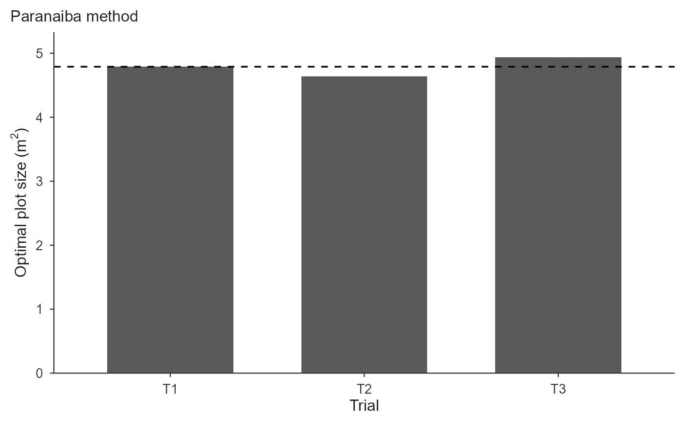
par_fit$summary
#> trial mean variance CV rho_row rho_col rho Xo
#> 1 T1 251.0129 3471.819 23.47375 0.01655932 0.09052249 0.01655932 4.793933
#> 2 T2 256.1666 3346.830 22.58366 0.14621177 0.10257518 0.14621177 4.638860
#> 3 T3 244.5397 3624.312 24.61861 0.08624510 0.10522436 0.08624510 4.936716
#> CVxo valid
#> 1 10.71956 TRUE
#> 2 10.37281 TRUE
#> 3 11.03883 TRUE
## rho is estimated along a serpentine walk. The original method walks the
## rows; walking the columns instead can give a visibly different Xo.
cbind(
row = calc_paranaiba(grids)$summary$Xo,
col = calc_paranaiba(grids, rho_direction = "col")$summary$Xo,
mean = calc_paranaiba(grids, rho_direction = "mean")$summary$Xo
)
#> Paranaiba method on 3 trial(s); rho direction = 'row'.
#> Paranaiba method on 3 trial(s); rho direction = 'col'.
#> Paranaiba method on 3 trial(s); rho direction = 'mean'.
#> row col mean
#> [1,] 4.793933 4.781240 4.789785
#> [2,] 4.638860 4.655951 4.648170
#> [3,] 4.936716 4.930684 4.933851
## Long format: one row per basic unit, with row and column indices
long <- data.frame(
trial = rep(uniformity_trial$trial, times = length(col_cols)),
row = rep(uniformity_trial$row, times = length(col_cols)),
col = rep(names(uniformity_trial)[col_cols], each = nrow(uniformity_trial)),
value = unlist(uniformity_trial[, col_cols], use.names = FALSE)
)
calc_paranaiba(long, value = "value", row_id = "row", col_id = "col",
trial = "trial")$summary
#> Paranaiba method on 3 trial(s); rho direction = 'row'.
#> trial mean variance CV rho_row rho_col rho Xo
#> 1 T1 251.0129 3471.819 23.47375 0.01655932 0.09052249 0.01655932 4.793933
#> 2 T2 256.1666 3346.830 22.58366 0.14621177 0.10257518 0.14621177 4.638860
#> 3 T3 244.5397 3624.312 24.61861 0.08624510 0.10522436 0.08624510 4.936716
#> CVxo valid
#> 1 10.71956 TRUE
#> 2 10.37281 TRUE
#> 3 11.03883 TRUE
# \donttest{
plot(par_fit)
 ## CVxo of each trial feeds the number of replications
calc_replicates(treatments = c(5, 10, 20),
cv_percent = mean(par_fit$summary$CVxo),
lsd_percent = c(10, 20))
#> Optimal number of replications
#> Design: CRD CV: 10.71% alpha: 0.05
#> Rows: 6 | Non-converged: 0
#>
#> Treatments CV_percent LSD_percent Alpha Design r_continuous r_optimal df_error
#> 5 10.7104 10 0.05 CRD 17.83 18 85
#> 10 10.7104 10 0.05 CRD 23.43 24 230
#> 20 10.7104 10 0.05 CRD 29.09 30 580
#> 5 10.7104 20 0.05 CRD 5.11 6 25
#> 10 10.7104 20 0.05 CRD 6.26 7 60
#> 20 10.7104 20 0.05 CRD 7.51 8 140
#> q_tukey converged at_floor
#> 3.942 TRUE FALSE
#> 4.519 TRUE FALSE
#> 5.035 TRUE FALSE
#> 4.153 TRUE FALSE
#> 4.646 TRUE FALSE
#> 5.110 TRUE FALSE
# }
## CVxo of each trial feeds the number of replications
calc_replicates(treatments = c(5, 10, 20),
cv_percent = mean(par_fit$summary$CVxo),
lsd_percent = c(10, 20))
#> Optimal number of replications
#> Design: CRD CV: 10.71% alpha: 0.05
#> Rows: 6 | Non-converged: 0
#>
#> Treatments CV_percent LSD_percent Alpha Design r_continuous r_optimal df_error
#> 5 10.7104 10 0.05 CRD 17.83 18 85
#> 10 10.7104 10 0.05 CRD 23.43 24 230
#> 20 10.7104 10 0.05 CRD 29.09 30 580
#> 5 10.7104 20 0.05 CRD 5.11 6 25
#> 10 10.7104 20 0.05 CRD 6.26 7 60
#> 20 10.7104 20 0.05 CRD 7.51 8 140
#> q_tukey converged at_floor
#> 3.942 TRUE FALSE
#> 4.519 TRUE FALSE
#> 5.035 TRUE FALSE
#> 4.153 TRUE FALSE
#> 4.646 TRUE FALSE
#> 5.110 TRUE FALSE
# }